
Knowing the top 10 most influential data mining algorithms is awesome.
Knowing how to USE the top 10 data mining algorithms in R is even more awesome.
That’s when you can slap a big ol' "S" on your chest...
...because you’ll be unstoppable!
Today, I’m going to take you step-by-step through how to use each of the top 10 most influential data mining algorithms as voted on by 3 separate panels in this survey paper.
By the end of this post...
You’ll have 10 insanely actionable data mining superpowers that you’ll be able to use right away.
UPDATE 18-Jun-2015: Thanks to Albert for the creating the image above!
UPDATE 22-Jun-2015: Thanks to Ulf for the fantastic feedback which I've included below.
[tocplus]Getting Started
First, what is R?
R is both a language and environment for statistical computing and graphics. It's a powerful suite of software for data manipulation, calculation and graphical display.
R has 2 key selling points:
- R has a fantastic community of bloggers, mailing lists, forums, a Stack Overflow tag and that's just for starters.
- The real kicker is R's awesome repository of packages over at CRAN. A package includes reusable R code, the documentation that describes how to use them and even sample data.
It's a great environment for manipulating data, but if you're on the fence between R and Python, lots of folks have compared them.
For this post, do 2 things right now:
The next step is to couple R with knitr…
Okay, what's knitr?
knitr (pronounced nit-ter) weaves together plain text (like you’re reading) with R code into a single document. In the words of the author, it’s “elegant, flexible and fast!”
You’re probably wondering...
What does this have to do with data mining?
Using knitr to learn data mining is an odd pairing, but it’s also incredibly powerful.
Here’s 3 reasons why:
- It’s a perfect match for learning R. I’m not sure if anyone else is doing this, but knitr lets you experiment and see a reproducible document of what you’ve learned and accomplished. What better way to learn, teach and grow?
- Yihui (the author of knitr) is super on top of maintaining, enhancing and making knitr awesome.
- knitr is light-weight and comes with RStudio!
Don’t wait!
Follow these 5 steps to create your first knitr document:
- In RStudio, create a new R Markdown document by clicking File > New File > R Markdown...
- Set the Title to a meaningful name.
- Click OK.
- Delete the text after the second set of
---. - Click
Knit HTML.
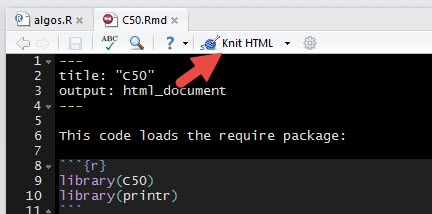
Your R Markdown code should look like this:
After “knitting” your document, you should see something like this in the Viewer pane:

Congratulations! You’ve coded your first knitr document!
Few pre-requisites
You'll be installing these package pre-reqs:
One final package pre-req is printr which is currently experimental (but I think is fantastic!). We're including it here to generate better tables from the code below.
In your RStudio console window, copy and paste these 2 commands:
Then press Enter.
Now let’s get started data mining!
C5.0
Wait… what happened to C4.5? C5.0 is the successor to C4.5 (one of the original top 10 algorithms). The author of C4.5/C5.0 claims the successor is faster, more accurate and more robust.
Ok, so what are we doing? We’re going to train C5.0 to recognize 3 different species of irises. Once C5.0 is trained, we'll test it with some data it hasn’t seen before to see how accurately it "learned" the characteristics of each species.
Hang on, what’s iris? The iris dataset comes with R by default. It contains 150 rows of iris observations. Each iris observation consists of 5 columns: Sepal.Length, Sepal.Width, Petal.Length, Petal.Width and Species.
Although we know the species for every iris, you’re going to divide this dataset into training data and test data.
Here’s the deal:
Each row in the dataset is numbered 1 through 150.
How do we start? Create a new knitr document, and title it C50.
Add this code to the bottom of your knitr document:
Can you see how plain text is weaved in with R code?
In knitr, the R code is surrounded at the beginning by a triple backticks. This tells knitr that the text between the triple backticks is R code and should be executed.
Hit the Knit HTML button, and you’ll have a newly generated document with the code you just added.
Note: The packages are loaded within the context of the document being "knitted" together. They will not stay loaded after knitting completes.
Sweet! Packages are being loaded, what’s next? Now we need to divide our data into training data and test data. C5.0 is a classifier, so you’ll be teaching it how to classify the different species of irises using the training data.
And the test data? That’s what you use to test whether C5.0 is classifying correctly.
Add this to the bottom of your knitr document:
Line 4 takes a random 100 row sample from 1 through 150. That’s what sample() does. This sample is stored in train.indeces.
Line 5 selects some rows (specifically the 100 you sampled) and all columns (leaving the part after the comma empty means you want all columns). This partial dataset is stored in iris.train.
Remember, iris consists of rows and columns. Using the square brackets, you can select all rows, some rows, all columns or some columns.
Line 6 selects some rows (specifically the rows not in the 100 you sampled) and all columns. This is stored in iris.test.
Hit the Knit HTML button, and now you’ve divided your dataset!
How can you train C5.0? This is the most algorithmically complex part, but it will only take you one line of R code.
Check this out:
Add the above code to your knitr document.
In this single line of R code you’re doing 3 things:
- You’re using the C5.0 function from the C50 package to create a model. Remember, a model is something that describes how observed data is generated.
- You’re telling C5.0 to use
iris.train. - Finally, you’re telling C5.0 that the Species column depends on the other columns (Sepal.Width, Petal.Height, etc.). The tilde means "depends" and the period means all the other columns. So, you’d say something like "Species depends on all the other column data."
Hit the Knit HTML button, and now you’ve trained C5.0 with just one line of code!
How can you test the C5.0 model? Evaluating a predictive model can get really complicated. Lots of techniques are available for very sophisticated validation: part 1, part 2a/b, part 3 and part 4.
One of the simplest approaches is: cross-validation.
What’s cross-validation? Cross-validation is usually done in multiple rounds. You're just going to do one round of training on part of the dataset followed by testing on the remaining dataset.
How can you cross-validate? Add this to the bottom of your knitr document:
The predict() function takes your model, the test data and one parameter that tells it to guess the class (in this case, the model indicate species).
Then it attempts to predict the species based on the other data columns and stores the results in results.
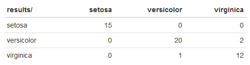
How to check the results? A quick way to check the results is to use a confusion matrix.
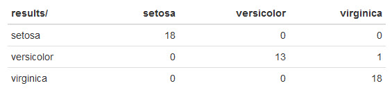
So... what’s a confusion matrix? Also known as a contingency table, a confusion matrix allows us to visually compare the predicted species vs. the actual species.
Here’s an example:
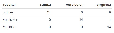
The rows represent the predicted species, and the columns represent the actual species from the iris dataset.
Starting from the setosa row, you would read this as:
- 21 iris observations were predicted to be
setosawhen they were actuallysetosa. - 14 iris observations were predicted to be
versicolorwhen they were actuallyversicolor. - 1 iris observation was predicted to be
versicolorwhen it was actuallyvirginica. - 14 iris observations were predicted to be
virginicawhen it was actuallyvirginica.
How can I create a confusion matrix? Again, this is a one-liner:
Hit the Knit HTML button, and now you see the 4 things weaved together:
- You’ve divided this iris dataset into training and testing data.
- You’ve created a model after training C5.0 to predict the species using the training data.
- You’ve tested your model with the testing data.
- Finally, you’ve evaluated your model using a confusion matrix.
Don't sit back just yet -- you've nailed classification, now checkout clustering...
k-means
What are we doing? As you probably recall from my previous post, k-means is a cluster analysis technique. Using k-means, we're looking to form groups (a.k.a. clusters) around data that "look similar."
The problem k-means solves is:
We don't know which data belongs to which group -- we don't even know the number of groups, but k-means can help.
How do we start? Create a new knitr document, and title it kmeans.
Add this code to the bottom of your knitr document:
Hit the Knit HTML button, and you’ll have tested the code that imports the required libraries.
Okay, what's next? Now we use k-means! With a single line of R code, we can apply the k-means algorithm.
Add this to the bottom of your knitr document:
2 things are happening on line 5:
- The
subset()function is used to remove theSpeciescolumn from the iris dataset. It's no fun if we know the Species before clustering, right? - Then
kmeans()is applied to the iris dataset (w/ Species removed), and we tell it to create 3 clusters.
Hit the Knit HTML button, and you’ll have a newly generated document for kmeans.
How can you test the k-means clusters? Since we started with the known species from the iris dataset, it's straight-forward to test how accurate k-means clustering is.
Add this code to the bottom of your knitr document:
Hit the Knit HTML button to generate your own confusion matrix.
What do the results tell us? The k-means results aren't great, and your results will probably be slightly different.
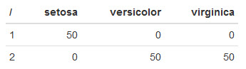
Here's what mine looks like:
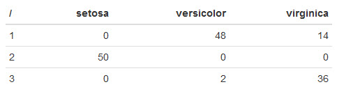
What are the numbers along the side? The numbers along the side are the cluster numbers. Since we removed the Species column, k-means has no idea what to name the clusters, so it numbers them.
What does the matrix tell us? Here's a potential interpretation of the matrix:
- k-means picked up really well on the characteristics for
setosain cluster 2. Out of 50setosairises, k-means grouped together all 50. - k-means had a tough time with
versicolorandvirginica, since they are being grouped into both clusters 1 and 2. Cluster 1 favorsversicolorand cluster 3 strongly favorsvirginica. - An interesting investigation would be to try clustering the data into 2 clusters rather than 3. You could easily experiment with the
centersparameter inkmeans()to see if that would work better.
Does this data mining stuff work? k-means didn't do great in this instance. Unfortunately, no algorithm will be able to cluster or classify in every case.
Using this iris dataset, k-means could be used to cluster setosa and possibly virginica. With data mining, model testing/validation is super important, but we're not going to be able to cover it in this post. Perhaps a future one... 🙂
With C5.0 and k-means under your belt, let's tackle a tougher one...
Support Vector Machines
What are we doing? Just like we did with C5.0, we’re going to train SVM to recognize 3 different species of irises. Then we’ll perform a similar test to see how accurately it “learned” the different species.
How do we start? Create a new knitr document, and title it svm.
Add this code to the bottom of your knitr document:
Hit the Knit HTML button to ensure importing the required libraries is working.
Loading of libraries is good, what's next? SVM is trained just like C5.0, so we need a training and test set, just like before.
Add this to the bottom of your knitr document:
This should look familiar. To keep things consistent, it's the same code we used to create training and testing data.
Hit the Knit HTML button, and you've divided your dataset.
How can you train SVM? Like C5.0, this is the most algorithmically complex part, but it will take us only a single line of R code.
Add this code to the bottom of your knitr document:
As in the C5.0 code, this code tells svm 2 things:
Speciesdepends on the other columns.- The data to train SVM is stored in
iris.train.
Hit the Knit HTML button to train SVM.
Let's test the model! We're going to use precisely the same code as before.
Add this to the your knitr document:
Hit the Knit HTML button to test your SVM model.
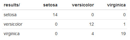
What do the results tell us? To get a better understanding of the results, generate a confusion matrix for the results.
Add this to the bottom of your knitr document, and hit Knit HTML:
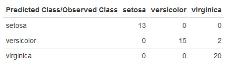
Here's what mine looks like:
The first thing that jumps out at me is SVM kicked butt!
The only mistake it made was misclassifying a virginica iris as versicolor. Although the testing so far hasn't been very thorough, based on the test runs so far... SVM and C5.0 seem to do about the same on this dataset, and both do better than k-means.
Now for my favorite...
Apriori
What are we doing? We're going to use Apriori to mine a dataset of census income in order to discover related items in the survey data.
As you probably recall from my previous post, these related items are called itemsets. The relationship among items are called association rules.
How do we start? Create a new knitr document, and title it apriori.
Add this code to the bottom of your knitr document:
Hit the Knit HTML button to import the required libraries and dataset.
Loading of libraries and data is working, what's next? Now we use Apriori!
Add this to the bottom of your knitr document:
This single function call does a ton of things, so let's break it down...
Line 4 tells apriori() that you'll be working on the Adult dataset and to store the association rules into rules.
Line 5 tells apriori() a few parameters it needs to filter the generated rules.
As you probably recall, support is the percentage of records in the dataset that contain the related items. Here you're saying we want at least 40% support.
Confidence is the conditional probability of some item given you have certain other items in your itemset. You're using 70% confidence here.
In truth, Apriori generates a ton of itemsets and rules...
...you'll need to experiment with support and confidence to filter for interesting rules/itemsets.
Line 6 tells apriori() certain characteristics to look for in the association rules.
Association rules look like this {United States} => {White, Male}. You'd read this as "When I see United States, I will also see White, Male."
There's a left-hand side (lhs) to the rule and a right-hand side (rhs).
All this line indicates is that we want to see race=White and sex=Male on the right-hand side. The left-hand side can remain the default (which means anything goes).
Hit the Knit HTML button, and generate the association rules!
How can you look at the rules? Looking at the association rules takes only a few lines of R code.
Add this code to the bottom of your knitr document:
Line 4 sorts the rules by lift.
What's lift? Lift tells you how strongly associated the left-hand and right-hand sides are associated with each other. The higher the lift value, the stronger the association.
Bottom line is: It's another measure to help you filter the large number of rules/itemsets.
Line 5 grabs the top 5 rules based on lift.
Line 6 takes the top 5 rules and converts them into a data frame so that we can view them.
Here's the top 5 rules:
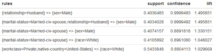
What do these rules tell us? When you're dealing with a large amount of data, Apriori gives you an alternate view of the data for exploration.
Check out these findings:
- In the 1st rule... When we see
Husbandwe are virtually guaranteed to seeMale. Nothing surprising with this revelation. What would be interesting is to understand why it's not 100%. 🙂 - In the 2nd rule... It's basically the same as the 1st rule, except we're dealing with
civilian spouses. No surprises here. - In the 3rd and 4th rules... When we see
civilian spouse, we have a high chance of seeingMaleandWhite. This is interesting, because it potentially tells us something about the data. Why isn't a similar rule forFemaleshowing up? Why aren't rules for other races showing up in the top rules? - In the 5th rule... When we see
US, we tend to seeWhite. This seems to fit with my expectation, but it could also point to the way the data was collected. Did we expect the data set to have morerace=White?
A word of caution:
Although these rules are based on the data and systematically generated, I get the feeling that there's a bit of an art to selecting support, confidence and even lift. Depending on what you select for these values, you may get rules that will really help you make decisions...
Alternatively...
You may get rules that mislead you.
But I have to admit, Apriori gives some interesting insights on a data set I didn't know much about.
Here's comes the toughest algorithm (at least for me)...
EM
What are we doing? Within the context of data mining, expectation maximization (EM) is used for clustering (like k-means!). We're going to cluster the irises using the EM algorithm. I found EM to be one of the more difficult to understand conceptually.
Here's some great news though:
Despite being difficult to understand, R takes care of all the heavy lifting with one of its CRAN packages: mclust.
How do we start? Create a new knitr document, and title it em.
Add this code to the bottom of your knitr document:
Hit the Knit HTML button to make sure you can import the required libraries.
All set, what's next? Now we use EM!
Add this to the bottom of your knitr document:
This should look familiar. We're removing the Species column (just like before), except this time we're using Mclust() to do the clustering.
Hit the Knit HTML button, and you've generated a cluster model using EM.
How are Mclust and EM related? Mclust() uses the EM algorithm under the hood. In a nutshell, Mclust() tunes a set of models using EM and then selects the one with the lowest BIC.
Hang on... what's BIC? BIC stands for Bayesian Information Criterion. In a nutshell, given a few models, BIC is an index which measures both the explanatory power and the simplicity of a model.
The simpler the model and the more data it can explain... the lower the BIC. The model with lowest BIC is the winner.
How can you test the EM clusters? You can test whether clustering was effective using the same approach as in k-means.
Add this code to the bottom of your knitr document:
Hit the Knit HTML button to generate your own confusion matrix.
Here's what mine looks like:
What are the numbers along the left-hand side? Just like k-means clustering, the algorithm has no idea what the cluster names are. EM found 2 clusters, so it numbered them accordingly.
Why only 2 clusters? Using the model selected by Mclust, this algorithm effectively segmented setosa from the other 2 species.
Like k-means, EM had trouble distinguishing between versicolor and virginica. While k-means had some success with virginica and to a lesser degree versicolor, k-means made the effort to form a 3rd cluster because we told it to form 3 clusters.
A neat feature of the mclust package is to plot the model. Here you can investigate the clustering plots:
Checkout the next algorithm which is used by Google...
PageRank
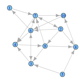
What are we doing? We're going to use the PageRank algorithm to determine the relative importance of objects in a graph.
What's a graph? Within the context of mathematics, a graph is a set of objects where some of the objects are connected by links. In the context of PageRank, the set of objects are web pages and the links are hyperlinks to other web pages.
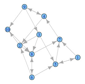
Here's an example of a graph:
How do we start? Create a new knitr document, and title it pagerank.
Add this code to the bottom of your knitr document:
Hit the Knit HTML button to try importing the required libraries.
Alright, what's next? Using the PageRank algorithm, the aim is to discover the relative importance of objects. Like k-means, Apriori and EM, we're not going to train PageRank.
Instead, let's generate a random graph to do our analysis:
The single line of R code in line 4 tells random.graph.game() 4 things:
- Generate a graph with 10 objects.
- There's a 1 in 4 chance of a link being drawn between 2 objects.
- Use directed links.
- Store the graph in
g.
What's a directed link? In graphs, you can have 2 kinds of links: directed and undirected. Directed links are single directional.
For example, a web page hyperlinking to another web page is one-way. Unless the 2nd web page hyperlinks back to the 1st page, the link doesn't go both ways.
Undirected links go both ways and are bidirectional.
What does this graph look like? Seeing a graph is so much better than describing a graph.
Add this code to the bottom of your knitr document:
Here's what mine looks like:
How can I apply PageRank to this graph? With a single line of R code, you can apply PageRank to the graph you just generated.
Add this code to the bottom of your knitr document:
The single line of R code applies the PageRank algorithm and retrieves the vector of PageRanks for the 10 objects in the graph. You can think of a vector as a list, so we're just retrieving a list of PageRanks.
How can I view the PageRanks? R already did the heavy lifting in order to calculate the PageRank of each object.
To view the PageRanks, add this code to the bottom of your knitr document:
Hit the Knit HTML button, and you’ll see the PageRanks.
Line 4 creates a data frame with 2 columns: Object and PageRank. You can think of a data frame as table with rows and columns.
The Object column contains the numbers 1 through 10. The PageRank column contains the PageRanks.
Bottom line is:
Each row in the data frame represents an object with its object number and PageRank.
Line 5 sorts the data frame from highest PageRank to lowest PageRank.
Here's what my data frame looks like:
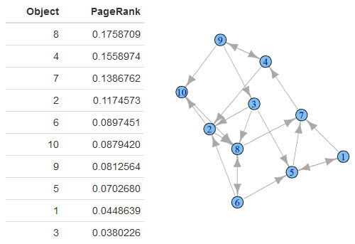
What does this table mean? This table tells you the relative importance of each object in the graph.
2 things are clear:
- Object 8 is the most relevant with a PageRank of 0.18.
- Object 3 is the least relevant with a PageRank of 0.04.
Looking back at the original graph, this seems to be accurate. Object 8 is linked to by 3 other objects: 3, 2 and 6. Object 3 is linked to by just object 9.
Remember, the number of objects linking to object 8 is just one component of PageRank...
...the relative importance of the objects linking to object 8 also factor into object 8's PageRank.
Ready for a boost?
AdaBoost
What are we doing? Like C5.0 and SVM, we’re going to train AdaBoost to recognize 3 different species of irises. Then we’ll perform a similar test on the test dataset to see how accurately it “learned” the different iris species.
How do we start? Create a new knitr document, and title it adaboost.
Add this code to the bottom of your knitr document:
Hit the Knit HTML button to test import of the required libraries.
Loading libraries is working, what's next? Just like before, we need a training and test set.
Add this to the bottom of your knitr document:
No change here. To keep things focused on the algorithms, it's the same code we used to create training and testing data.
Hit the Knit HTML button, and you now have a training and test dataset.
How can you train AdaBoost? Just like before, this will take us only a single line of R code.
Add this code to the bottom of your knitr document:
As before, this code tells adaboost 2 things:
Speciesdepends on the other columns.- The data to train AdaBoost is stored in
iris.train.
Hit the Knit HTML button to train AdaBoost.
Why does AdaBoost take longer to train? R's default number of iterations is 100. You can modify the number of iterations using the mfinal parameter.
As you'll recall from AdaBoost in plain English, AdaBoost is trained in rounds (a.k.a. iterations).
You might be wondering:
If AdaBoost consists of an ensemble of weak learners...
What are the weak learners? boosting() is an implementation of AdaBoost.M1. This variation uses 3 weak learners: FindAttrTest, FindDecRule and C4.5.
How do you test the model? Let's use precisely the same code as before.
Add this to your knitr document:
Hit the Knit HTML button to test your AdaBoost model.
What do the results tell us? To get a better understanding of the results, output the confusion matrix for the results.
Add this to the bottom of your knitr document, and hit Knit HTML:
Here's what mine looks like:
AdaBoost did well!
It only made 2 mistakes misclassifying 2 virginica irises as versicolor. A single test run isn't a lot to thoroughly evaluate AdaBoost on this dataset, but this is definitely a good sign.
The next algorithm might be lazy, but it's definitely no slouch...
kNN
What are we doing? We’re going to use the kNN algorithm to recognize 3 different species of irises. As you'll recall from my previous post, kNN is a lazy learner and isn't "trained" with the goal of producing a model for prediction.
Instead, kNN does a just-in-time calculation to classify new data points.
How do we start? Create a new knitr document, and title it knn.
Add this code to the bottom of your knitr document:
Hit the Knit HTML button to try importing the required libraries.
All set, what's next? Despite that you're not "training" kNN, the algorithm still requires a training set to base its just-in-time calculations on. We'll need a training and test set.
Add this to the bottom of your knitr document:
Hit the Knit HTML button, and you now have a training and test dataset.
How do you use kNN? In just a single call, you'll be initializing kNN with the training dataset and testing with the test dataset.
Add this code to the bottom of your knitr document:
This code tells kNN 3 things:
- The training dataset with the Species removed.
- The test dataset with the Species removed.
- The Species of the training dataset is specified by
clwhich stands for class.
Hit the Knit HTML button to get the prediction result.
What do the results tell us? To get a better understanding of the results, output the confusion matrix for the results.
Add this to the bottom of your knitr document, and hit Knit HTML:
Here's what mine looks like:
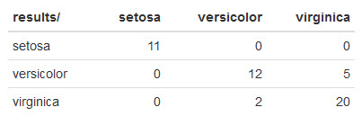
kNN made a few mistakes:
- It misclassified 5
virginicairises asversicolor. - In addition, it misclassified 2
versicoloririses asvirginica.
Not as great as some of the other results we've been seeing, but pretty decent since we're using the default kNN settings.
The next algorithm may be naive, but don't underestimate it...
Naive Bayes
What are we doing? We’re going to use the Naive Bayes algorithm to recognize 3 different species of irises.
How do we start? Create a new knitr document, and title it nb.
Add this code to the bottom of your knitr document:
Hit the Knit HTML button to try importing the required libraries.
Cool, what's next? We'll need a training and test set.
Add this to the bottom of your knitr document:
Hit the Knit HTML button, and you now have a training and test dataset.
How can you train Naive Bayes? Just like before, this will take us only a single line of R code.
Add this code to the bottom of your knitr document:
This code tells naiveBayes 2 things:
- The data to train Naive Bayes is stored in
iris.train, but we remove theSpeciescolumn. This isx. - The
Speciesforiris.train. This isy.
Hit the Knit HTML button to train Naive Bayes.
How do you test the model? We'll use precisely the same code as before.
Add this to the your knitr document:
Hit the Knit HTML button to test your Naive Bayes model.
What do the results tell us? Let's output the confusion matrix for the results.
Add this to the bottom of your knitr document, and hit Knit HTML:
Here's what mine looks like:
Naive Bayes did quite well!
It made 2 mistakes misclassifying 2 virginica irises as versicolor and another mistake misclassifying versicolor as virginica.
Last, but not least...
CART
What are we doing? In this last and final algorithm, we’re going to use CART to recognize 3 different species of irises.
How do we start? Create a new knitr document, and title it cart.
Add this code to the bottom of your knitr document:
Hit the Knit HTML button to see if importing the required libraries works.
What's next? CART is a decision tree classifier just like C5.0. We'll need a training and test set.
Add this to the bottom of your knitr document:
Hit the Knit HTML button, and you now have a training and test dataset.
How can you train CART? Once again, R encapsulates the complexity of CART nicely so this will take us only a single line of R code.
Add this code to the bottom of your knitr document:
This code tells CART 2 things:
Speciesdepends on the other columns.- The data to train CART is stored in
iris.train.
Hit the Knit HTML button to train CART.
How do you test the model? We'll be using predict() again to test our model.
Add this to the your knitr document:
Hit the Knit HTML button to test your CART model.
What do the results tell us? The confusion matrix for the results is generated in the same way.
Add this to the bottom of your knitr document, and hit Knit HTML:
Here's what mine looks like:
The default CART model didn't do awesome compared to C5.0. However, this is a single test run. Performing more test runs with different samples would be a much more reliable metric.
In this particular case, CART misclassified 1 virginica iris as versicolor and 4 mistakes misclassifying versicolor as virginica.
You Can Totally Do This!
Right now, I want you to do one thing:
Pick one one of these algorithms, and commit to giving it a try right now.
Leave a comment about which algorithm you picked. If you want, you can even mention why.
Then...
Take action, and try out the algorithm.
Did you get slightly different results? Did you run into any issues?
Let me know what you think by leaving a comment.
Comments 30
Great to see another post for beginners like me.
I had a quick look and planning to start doing the pagerank implementation this weekend
My pleasure, Lakshminarayanan! Would love to hear how it goes for you. 🙂
Very very nice.. indeed, congratulations!
Remark about the package requisites: both ‘class’ and ‘rpart’ already *come* with every regular R installation. It makes sense therefore to *exclude* them from the “list” you pass to `install.packages(.)`.
Appreciate it, Martin! 🙂
Thanks for the pre-reqs remark. It’s corrected now.
From a brief review, for me it would be best to start with
“First, what is R” and then all the rest. Anyway, looks
like a great reference for data mining experiments.
Thanks, Ilan. It’s a good point about explaining R. I added a bit of context around what R is now. 🙂
Ray – Thanks very much for creating this. This is definitely a quick start for beginners like me. This post combined with your earlier post on the same topic is awesome for someone to get started with ML using R. Simple, Straightforward explanations – I love it…
My only request to you is to do something similar to help learn the basics of R. Your post does a good job of explaining the ML aspects of the script, but would love to immerse into R as well.
My pleasure, Suresh! That’s a fascinating idea about learning the basics of R. I’ll definitely keep it in mind for a future post.
Thanks for the examples! Makes for a great reference of starting points when building models. Do you have any plans for a post for exploratory visualization of data? Things like PCA or autoencoders, charts to show clustering or the support vector for SVM, etc. Perhaps a comment about scikit-learn?
My pleasure, Daniel.
I considered adding visualization of the clustering/classification, but left it out to keep things super straight-forward. I absolutely agree that it’s important though. Regarding the scikit-learn Python library, I’m getting the sense the algorithms deserve a similar post for Python. I know a lot of the readers/subscribers also use Python.
Pingback: Top 10 data mining algorithms in plain R « Another Word For It
Hi Ray!
[ R and Rstudio latest version,
under Linux Ubuntu 12.04, 32-bits ]
ALL required pkgs
downloaded OK
and are shown (with [ ] checkboxes unmarked) ,
in the [Packages] tab of Rstudio.
But, as you instructed,
when I added these lines below (enclosed by 3 backticks: “`)
to my Knitr doc:
This code loads the required packages:
“`{r}
library(C50)
library(printr)
“`
then the html doc is rendered ok
in my Rstudio Viewer pane,
BUT…
the C50 and printr Packages are NOT loaded…
(ie: the Packages pane in Rstudio
shows [ ] empty checkboxes next to each Pkg. name…).
The Knitr pkg IS loaded,
BUT the C50 and the printr pkgs are NOT loaded.
What should I try next? HELP!
RaySF
Hi RaySF,
No problem. The packages load within the context of “knitting” and will not stay loaded after the HTML doc is rendered.
The knitr package is likely loaded through RStudio by default.
I’ll make some tweaks to the post to make the “knitting” thing clearer.
Ray
Thanks Ray#1 !!!
It’s _exactly_ what you said.
I misinterpreted your instructions at that point…
Everything works ok.
What a wonderful and clear article
…Great!
(Starbucks coffee is on me, next time I go by Seattle…)
RaySF
Thanks, RaySF. 🙂
Pingback: ã€æ•°æ®æŒ–掘】å大ç»å…¸æ•°æ®æŒ–掘算法Rè¯è¨€å®žè·µï¼ˆäº”) | 王路情åšå®¢—æ•°æ®ç§‘å¦å®¶
Pingback: å大ç»å…¸æ•°æ®æŒ–掘算法Rè¯è¨€å®žè·µï¼ˆå…«ï¼‰ | 王路情åšå®¢—æ•°æ®ç§‘å¦å®¶
Pingback: ã€æ•°æ®æŒ–掘】å大ç»å…¸æ•°æ®æŒ–掘算法Rè¯è¨€å®žè·µï¼ˆä¹ï¼‰ | 王路情åšå®¢—æ•°æ®ç§‘å¦å®¶
Ray,
Would you plan on building a similar post for Python?
Also, where does feature extraction and feature engineering come in this process?
Does the train() method handle that internally? I was under the assumption that feature engineering was one of the toughest parts to solve
I am totally new and potentially naive to machine learning
I’m considering doing a similar post for Python. No specific plans on when yet though.
Feature extraction and feature engineering would in most cases come before the use of these algorithms. Some of the more “exploratory” algorithms could be used to point you in the direction of interesting features (e.g. the clustering or association ones).
Unfortunately, I’m unfamiliar with the train() method. However, I did a quick search, and I’m assuming you’re referring to the caret package. Looking quickly at the docs, I don’t believe the train() method does feature extraction/engineering. Automating extraction/engineering is a difficult problem, and I’m pretty sure train() expects you’ve already selected/designed your features before training your model.
Thank you is not enough for you. I love your style and learnt a lot from this post. Please keep the good work and present more algorithm with its coding in R.
Thank you for the kind words, dhaif. Glad you found the post useful.
first thanks a lot for such a nice post, i am using text mining most of the time using NB.
if you can post something related to text mining it will be great !!
Thanks again for excellent post.
I am writing my bachelor thesis about Classification algorithms and I’m doing an applied part although I don’t know much about R (I study business). This post was a complete lifesaver for me ! It’s a great start for beginners. Thank you so much for doing this !
Hi Ray –
This is THE BEST Machine Learning article of all.
I sincerely mean it.
A lingering doubt –
each time I run the iris examples
(using C5.0, Knn or other algos),
the Confusion Matrix yields a slightly different accuracy result.
I guess that’s due
to the necessary _random sampling_ of the iris dataset,
into a “train” and “test” subsets.
That makes it difficult to decide
which algo is “better” (more accurate)
on a certain data set, (ie: iris).
Q:
===
– Is there a way
to have a more firm, stable [Confusion Matrix] results
for each algo,
(to allow deciding which algo is really better
for a certain dataset?).
Ray, hope you can shed some of your wise photons
on this matter! 🙂
RaySF
confused by the different [Confusion Matrix] results,
each time I run an algo…
first a BIGGGGG thanks to you.
Man wonderful teaching with code ,I never found this best anywhere.
Please do post more like this ,we have lots of followers for your post.
wonderful and excellent post.
Hi! For the mclust part,
the model always selects the highest BIC instead of the lowest one. For instance,
Top 3 models based on the BIC criterion:
VEV,2 VEV,3 VVV,2
-561.728462114339 -562.551437983528 -574.017832269830
These values above the top 3 and it chooses VEV with 2 clusters. You can also get it running the “model” itself.
The difference is that the BIC score used here is the negation of the BIC score defined on the wikipedia. You should be maximizing the model scores whereas using the BIC score as defined on the wikipedia you should be minimizing the score.
So the model selects the one with highest score.
sir gudafternoon
thank u very much for ur nice teaching of R tool for beginners like me
by reading this i wish to learn R tool thoroughly
i request u to post some more guidance to know thoroughly
Ray,
Pingback: How retargeting algorithms help in web personalization
Thank you very much for this blog post. I’m trying to learn R programming and statistics on my own in order to analyze crime data. I’m not exactly sure if I’ll be using any of the methods you shared for crime data analysis, but I know those methods will come in handy.